Unlocking Subsurface Value with GeoSoftware Professional Services
Read More

Time-lapse seismic technology was first introduced to the oil and gas industry by Arco in the early 1980s, and the commercial boom happened when the technique was successfully applied to North Sea fields in the late 1990s and early 2000s. The technology mainly consists of repeating 3D seismic surveys at different time intervals to image fluid and pressure (or temperature) changes during hydrocarbon production. The success of repeat seismic surveys involves identifying the undrained areas of hydrocarbon fields or the areas of steam injection.
During the last two decades, the evolution of 4D technology through advances in seismic acquisition, processing, and interpretation, has increased its role in monitoring the life cycle of a field and positioned the 4D method as the mainstream and most practical tool in reservoir monitoring and field management.
The value of 4D seismic was discussed by J.P. Blangy et al. (2017), in which the authors used a diagram (Figure 1) to show the value of using the 4D seismic throughout the life of a field and its use of optimal field management. In Figure 1, the vertical axis reflects cash flow as a function of time, and the areas shaded in red are times of negative cash flow. The field produces until cash flow falls below operating expense, at which point the field is abandoned. There are four overlapping phases where 4D seismic, as part of an integrated reservoir surveillance program, can bring value throughout the life-of-field development.
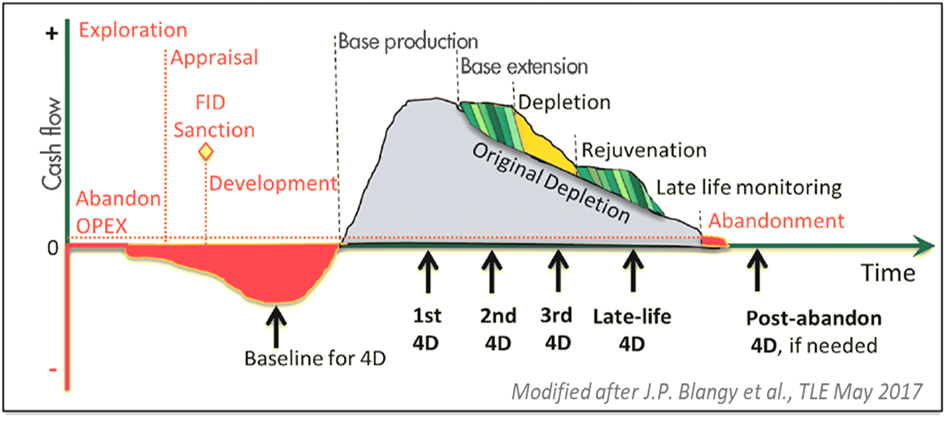
Figure 1: Four phases of the life cycle of an oil field: (1) base production/injection and its extension, (2) depletion, (3) rejuvenation, and (4) late-life/pre-abandonment. For each phase, a prudent operator will assess the viability of acquiring a new (4D) seismic data set.
The business impact of 4D seismic is best described as increasing an asset's Net Present Value (NPV), improving the well success rates, reducing the drilling cost, booking additional reserves, and prolonging the field life.
Ian Jack (2017) demonstrated the business impact of 4D through real examples from North Sea fields. One of the early business impacts is that Statoil (now Equinor) in 2004 reported the NPV of their 4D technology on the Gullfaks reservoir after five 4D surveys was USD$505 million. By 2006, six 4D surveys had been recorded, additional wells had been drilled, and the figure had increased to $992 million. The report also pointed out that 50% of the calculated NPV of each well drilled was allocated to the 4D data. By 2008, the 4D-based savings for Gullfaks alone approached $1 billion, and on average, there was a 6% reduction in drilling costs and additional reserves amounting to an average of 5% per field.
The 4D signal usually is 10 -100 times weaker than the primary signal, so the success of the 4D project is determined by detectability and repeatability factors. Oil and Gas operators often run screening and feasibility analyses to determine better the success rate of a 4D project, the magnitude and interoperability of the 4D seismic response, the optimal timing of repeat surveys, and the expected cost/benefits of acquiring 4D surveys.
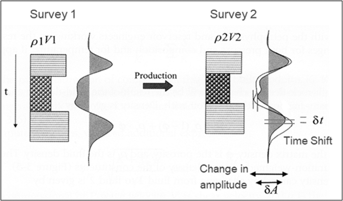 Figure 2: Feasibility analysis helps understand the expected seismic response from possible production-induced changes.
In a study of the producing Alpha oil field, located in the West African deep offshore, Bruce Webb et al. (2019 & 2020) performed a 4D feasibility study to assess and verify the sustainability and benefits of a 4D seismic acquisition. The feasibility study consisted of two phases. First, a Petro-Elastic Model (PEM) was computed based on the well data and laboratory ultrasonic tests. Then the seismic response was simulated for different production scenarios and analyzed at selected well locations. An evaluation of the detectability and measurability of the 4D signal in the presence of noise was done by adding random noise to the synthetic gathers and computing the associated Normalized Root Mean Square (NRMS). The authors concluded that the well-based 4D feasibility could clearly recognize production-induced 4D signals due to changes in fluid saturation, both in terms of amplitude/acoustic impedance changes and time shifts, even in the presence of a 30% NRMS noise level. However, the well-based 4D feasibility is usually limited in addressing the lateral-sweep interpretation or timing of the repeat surveys. Hence, the second phase was implemented, and a 4D time-lapse modeling allowed for deriving 3D elastic parameters and synthetic seismic volumes at selected production time steps. The modeling considered two different dynamic reservoir models to simulate relevant alternative scenarios: one in which the main faults displayed a leaking behavior and another in which the same faults are considered as seals (Figure 3). Both scenarios were consistent with the available production data at that time. The authors (Bruce Webb et al. 2019 & 2020) concluded that the 4D feasibility study helped estimate the mechanism and the magnitude of the 4D effect and generated a framework for interpreting and employing the 4D data once acquired.
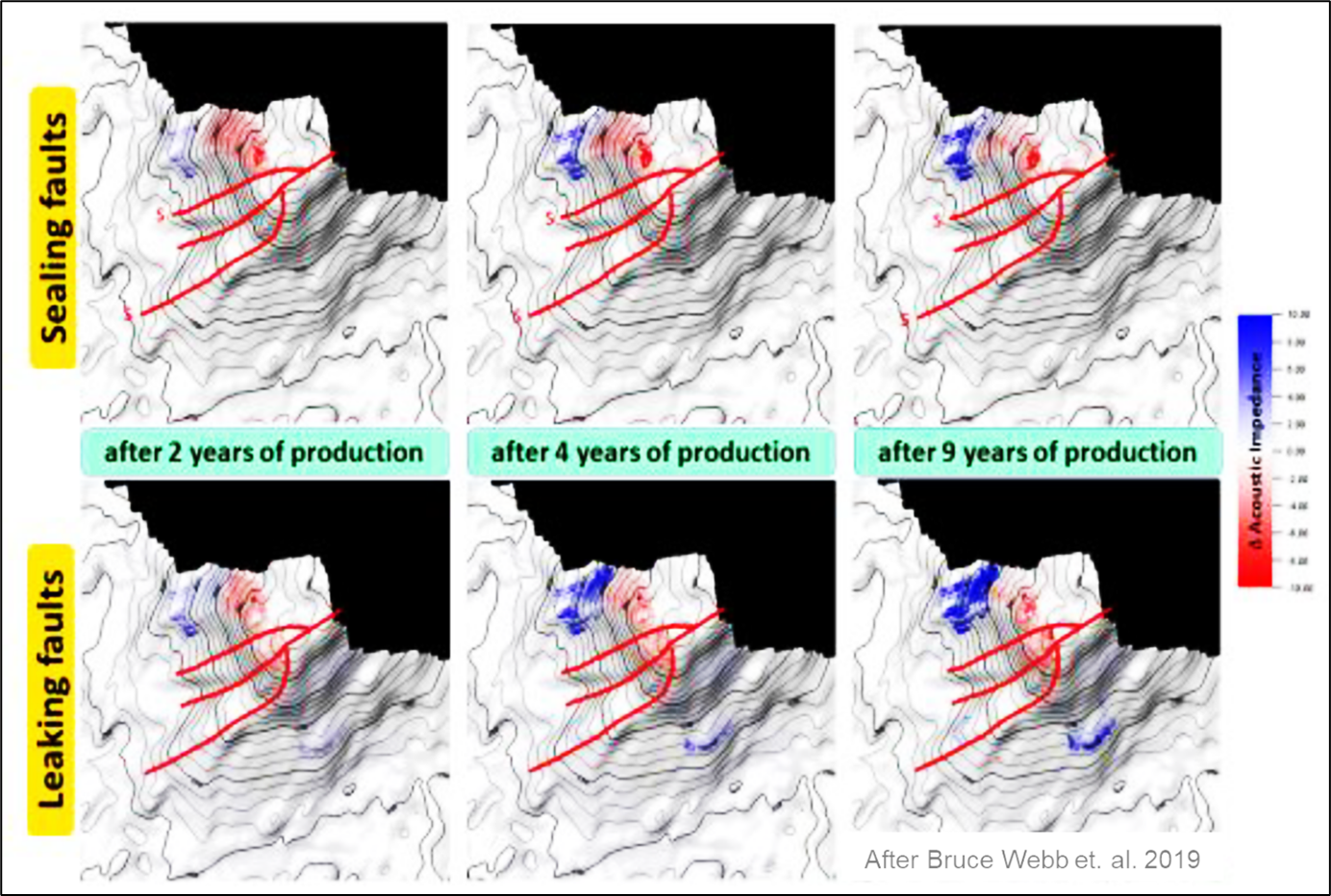
Figure 3: Alternative geological scenarios of sealing and leaking after years of production (after Bruce Webb et al. 2019).
Seismic repeatability is critical to minimize 4D interpretation uncertainty and maximize 4D project success. Sources of non-repeatable noise often include acquisition-geometry differences, sources and recording types of equipment, overburden complexity, static shifts, imaging parameters, ambient noise, and other environment-based noise such as sea tides, water temperature/salinity, rigs/structure, etc.
The acquisition and processing of seismic data should ensure the repeatability of a seismic event at nonproductive zones. A common approach to addressing non-repeatability noise sources is by applying a series of cross-equalization and data conditioning steps, focusing on the non-producing zones (above and below the reservoir) to ensure the only differential signal is at the reservoir level (producing zone).
The most common measures of repeatability are the Normalized RMS difference (NRMS) and the predictability (PRED), both of which are discussed by Kragh and Christie (2002). Using NRMS in conjunction with the RMS difference and RMS amplitude ratio is also a common procedure.
Another measure of repeatability is quality and anomaly, as discussed by Coleou et al. (2013), Quasicorrelation (accounting for both amplitude and phase difference) and Signal-to-Distortion ratio (SDR described by Cantillo 2011) are additional attributes for similarity measurement.
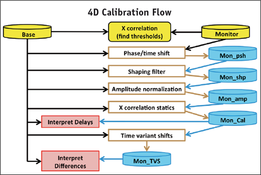
Figure 4: The 4D calibration flow includes: cross-correlations and cross-plots of seismic volumes and a comparison of volumes using a differencing tool; volume matching by time & phase matching, shaping filter, amplitude crossnormalization, and time-variant shifts (image modified from HampsonRussell Pro4D).
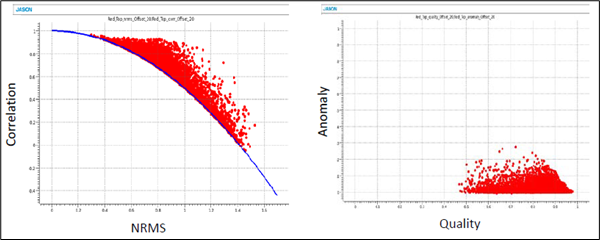 Figure 5: Repeatability measurements: cross plot of NRMS vs. cross-correlation (left) and Quality vs. Anomaly (right) are two complementary methods in displaying the similarity between two data volumes (image modified from Jason Workbench tutorial).
One of the key calibration steps is finding the optimal time shifts to calibrate the monitor surveys with the base survey. In addition, it provides a means for making incremental improvements to repeatability and offers a method for producing many final 4D interpretation products (David Johnston, 2013). Traditionally, this is done using standard cross-correlation methods. However, several other options have been developed in HampsonRussell Pro4D for computing the time shifts, such as the Taylor series expansion method, dynamic time warping, and vector warping with Gaussian windowing (Figure 6).
Naeini et al. (2009) described a multi-vintage time-shift estimation procedure that was based on earlier work by Hatchell et al. (2007). They assumed two vintages of seismic time-lapse data differ by a time shift that can be written as a Taylor series expansion. They showed how to minimize the problem by setting the derivative of the Taylor series with respect to the time shift equal to zero and then computing the shifts simply from the traces and their first derivatives.
Dynamic time warping (DTW) was first developed for voice recognition by Sakoe and Chiba (1978) in their paper “Dynamic programming algorithm optimization for spoken word recognition.” Their algorithm was used to stretch and squeeze speech to match the stored voice pattern in phone conversations. Dave Hale (2013) adopted the algorithm for seismic processing and pointed out that this method is more accurate than the cross-correlation method when the time shifts vary rapidly.
The injection of heat or fluids into the reservoir will also affect the horizontal stresses and create inline and crossline shifts (Guilbot and Smith, 2002). The vector warping method (apparent displacement vectors – Dave Hale 2009) allows for estimating the shifts in all three directions.
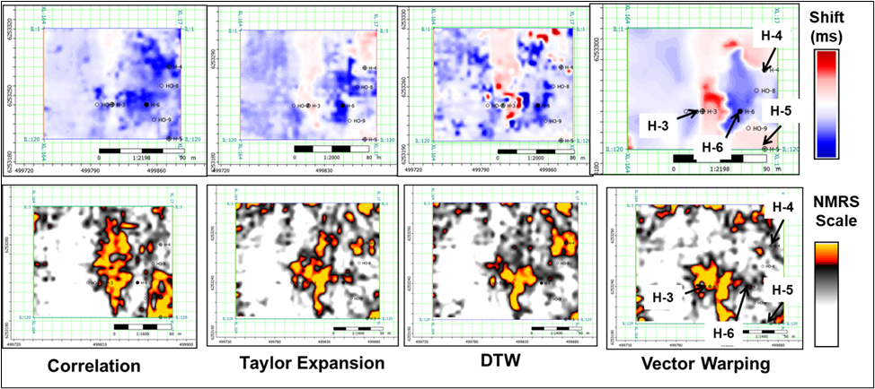
Figure 6: Time shifts (top) and NRMS amplitude difference (bottom) comparison of Base minus Monitor 3 over a steamflood case study, GLISP pilot, Northern Alberta (adopted from Brian Russell’s talk 2023). Noting that H-6 was the main injector in the second two time periods and that H-3, H-4, and H-5 had been converted to producers after time period 1. The comparison shows that Taylor expansion, DTW, and Gaussian correlation results are more consistent than the conditioned cross-correlation.
Another way of aligning the different vintages and estimating the time shifts is by aligning the seismic data of each vintage to the synthetic outputs generated during Jason RockTrace seismic inversion process. This synthetic method significantly reduces the mismatch between volumes with sub-sample accuracy.
The idea behind aligning over inverted synthetic seismic angle stacks modeled in the inversion process is that they are time-compatible, as all angle stacks are modeled from the same input set of elastic properties. This approach could be used to align 3D partial stacks prior to seismic inversions, estimate the time shifts of multiple 4D surveys, or register the PS to PP seismic data. Andrea Damasceno et al. (2022) used that synthetic method to improve the PS to PP time registration in a time-lapse PP-PS study over the Jubarte field, offshore Brazil. As long as the initial alignment is reasonable, the synthetic method can refine it to sub-sample accuracy since the synthetics created by the inversion process will always be perfectly aligned.
Baytok et al. (2017) showed the value of applying cross-equalization workflow over two land seismic vintages (4D) of low repeatability prior to a pre-stack seismic inversion and 4D interpretation (Figure 7). In this study, different vibrators were used for the base (2002) and monitor (2011) surveys. However, the monitor survey was designed to emulate the baseline acquisition parameters as closely as possible and parallel processing was maintained for both surveys. The work aimed to investigate undrained liquid gas pockets and to help with the planning of gas storage in depleted reservoirs in Central Thrace Basin, Turkey. The authors successfully applied four- equalization steps to angle stack vintages: (1) phase and time matching, (2) shaping filter, (3) cross-correlation time shifts, and (4) time-variant statics.
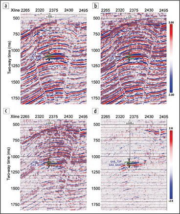
Figure 7: (a) 2002 base survey and (b) 2011 monitor survey crossline stack seismic sections and corresponding
differences (c) before and (d) after cross-equalization. The black curve is Sw (value decreases to the left). Green markers indicate the top and base of the gas interval. After applying the cross-equalization workflow, the nonproduction-related differences are removed from the difference section (after Baytok et al. 2017).
Summary
Here are some takeaways from today’s article:

To learn more about how GeoSoftware's reservoir experts can help you with your next 4D project, visit our Services page.

AUTHOR: Mohammed Ibrahim, Global Services Manager
Mohammed has over 20 years of experience in the oil and gas industry, most notably in geostatistical seismic inversion, QI geophysics, 4D seismic, and azimuthal seismic analysis. He has a proven record in integrating large, multi-scale, multi-disciplinary data to characterize hydrocarbon reservoirs and build “what-if” scenarios for both exploration and production fields. Mohammed has worked globally with NOCs, IOCs, and super-major oil and gas companies in a wide variety of complex petroleum provinces in North and Latin America, the Atlantic margins, the Middle East, and Western Australia. Mohammed holds a Ph.D. degree in geophysics from Michigan Technological University, and he currently oversees the professional services function within GeoSoftware.